Importance of Design of Tidal Stream Farms
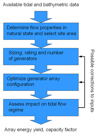
Fig. 1 – Processes involved in assessing the optimal power output of a tidal stream generator array.
Resource assessment forms part of the design process for an array of tidal stream generators – as indicated in the flow diagram in Figure 1 – and consists of the following tasks:
-
Selection of sites suitable for placing of tidal stream generator arrays. This is primarily constrained by a minimum value of mean cube flow speed (For a fixed generation efficiency, this value will be proportional to the average power output for a single turbine.); and a suitable range of depths for a particular type of generator. Site selection will also be constrained by integration with the power distribution network and environmental impact.
-
Initial sizing and rating of the generating device to maximize energy extracted over the life of the device taking into account factors such as the long term variations in flow speed; deviation of the flow from rectilinear movement; vertical profile of flow velocity.
-
Investigation of different arrangements of generators within the selected area given the device parameters above, in order to maximize combined power output. Revision of generator parameters if necessary.
-
Investigation of the geographical extent of significant effect of the proposed tidal stream generator array on tidal parameters (extracting tidal energy in one location may lead to a reduction in available energy elsewhere). If necessary, corrections made to power output estimates due to resulting changes in boundary conditions.
Table 1 – Methods for generating tidal flow data for use in resource assessments. 1, 2 and 3-D models can also be used to assess the effect of the generator arrays on the tidal regime, whereas previous assessments have used empirical corrections to flow values in the natural state to take account of the effect of multiple generators.
|
Tidal flow data
|
Advantages
|
Disadvantages
|
|
Nearest representative values from navigational charts
|
Simple, data easily obtainable.
|
Inaccurate over large areas and with sparse data. Corrections made for effects of generators can only be included empirically.
|
|
Interpolate between data points
|
Simple, more accurate than above.
|
Doesn’t account for changes in flow due to depth and other effects.
|
|
1D model
|
Simple, suitable for ‘fences’ of generators across well-defined channels. May be solved analytically.
|
Not suitable for complex topography. Can not simulate flow acceleration between generators.
|
|
2D numerical model
|
Well established for coastal tidal modelling. Energy extracted through added roughness.
|
Increasing computational expense. 3-D Wake structure not simulated. Requires tuning and validation.
|
|
3D numerical model
|
Can simulate wakes of turbines and include vertical velocity profile.
|
Complex. Currently suitable only for highly localized models. Data may be lacking on turbulence quantities.
|
Table 2 – Tidal stream energy resource for five sites in the Channel Islands according to three different reports.
|
Black and Veatch, 2004
|
Joule 2, 1996
|
ETSU, 1993
|
||||||
| Tidal Race |
Area
|
Max. Speed
|
Rated Power
|
Load Factor
|
Rated Power
|
Load Factor
|
Rated Power
|
Load Factor
|
|
km²
|
m/s
|
MW
|
%
|
MW
|
%
|
MW
|
%
|
|
| Race of Alderney |
102
|
4.4
|
394
|
49
|
1973
|
44
|
2407
|
23
|
| Casquets |
190
|
2.6
|
538
|
35
|
370
|
50
|
2943
|
13
|
| NW Guernsey |
222
|
2.1
|
170
|
33
|
422
|
54
|
2186
|
22
|
| Big Russel |
59
|
2.6
|
101
|
43
|
219
|
47
|
1001
|
22
|
| NE Jersey |
58
|
3.1
|
57
|
33
|
196
|
45
|
1179
|
13
|
Previous Estimates
Assessments of the tidal stream energy resource have taken the form of desktop studies, produced using navigational data, for the purpose of providing government and industry with broad estimates of the economic potential for the development of tidal stream power.
Recent assessments of tidal stream energy resources around the UK have estimated the exploitable resource, when averaged over a year, in the range 2 – 7 GW, which may be compared to an average electrical power consumption in the UK for 2005 of 46 GW (Digest of UK energy statistics 2006). There is considerable uncertainty attached to these resource estimates, however; all of the assessments to date have either ignored the change in flow conditions due to the effect of the generating devices, or have been based on more or less arbitrary proportions of kinetic energy flux through a site.
Fig. 2 – Part of a finite element mesh used for modelling tidal flows around Portland Bill, with sea bed elevations in metres above chart datum (scale on right). Co-ordinates are OSGB National Grid.
The results from three reports for the five key sites in the Channel Islands (shown in maps.live.com) are shown in Table 2 above. This clearly highlights a large discrepancy between reports and a need to make more accurate estimates of the resource.
Modelling of Tidal Currents
Portland Bill on the South coast of the UK (view in maps.live.com) is a promising site for tidal stream energy, with high tidal stream velocities of up to seven knots (3.6 m/s) around the headland. Although the area with high tidal streams is smaller than other proposed sites in Scotland or the Channel Islands, the location is closer to population centres than these sites.
Fig. 3 – Tidal flows around Portland Bill headland. Colour scale is in m/s and vectors show direction and relative magnitude of the velocity field. Rectangle shows the approximate area with highest average flow speed (actually highest mean cube speed).
In order to produce high resolution data on tidal streams, independent of navigational charts, a 2D tidal hydrodynamic model of this promising site has been produced using the TELEMAC system. The model was forced by tidal elevations around the outer boundary and the results validated using tidal elevation records at Weymouth (within the model domain) and tidal diamonds from the relevant Admiralty charts. One of the finite element meshes used for the model can be seen in Figure 2, along with the bathymetry of the area. Some of the results of the model can be seen in Figure 3 and the animation of tidal flows around the headland below.
Work has been published in:
Blunden L.S. and Bahaj A.S. (2006) Initial evaluation of tidal stream energy resources at Portland Bill, UK. Renewable Energy, Volume 31, Issue 2, February 2006, pp 121-132. View paper.
Forecasting
Fig. 4 – 28 day prediction for speed and direction from TELEMAC simulation.
For example tidal data, simulation results around Portland Bill have been used, this site has a significant swing from the 180º flow reversal, allowing comparisons between fixed orientation and yawing devices. The variation of depth-averaged speed over 28 days from the simulation is shown in Figure 4.
The T_TIDE package for MATLAB was used to determine the constituent ellipse properties by harmonic analysis, in which nodal corrections were applied, based on the central time of the input time series. Based on the solved constituents, predictions can be made from any start date with any time step. For the predictions in this paper, the tidal stream speeds and directions from the start of 2006 for 18 years have been generated at one minute intervals.
Fig. 5 – Hodograph showing direction and strength of the tidal flow. The first 5 days are the black lines and the shaded gray area represents the full 18 year forecast.
A hodograph showing a forecast for 18 years is presented in Figure 5 and first 5 days are shown to demonstrate a typical cycle. The ellipse is offset south due to the constant flow component. This and the constituents with inclination close to 0° or 90° cause the tidal stream to swing away from rectilinearity.
Some marine current turbine concepts do not turn to face the tide and instead rely on the tidal stream at the site to be bi-directional. Thus the rotor orientation is fixed but the blades are able to twist through 180 degrees capturing the energy by running the generator backwards. For this case direction is also important.
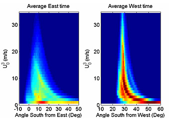
Fig. 6 – Binned data set showing a histogram of the times in the east and west. (Red denotes higher number of hours). The bins are defined by 1° intervals and in cubed speed steps of 1 m3/s3 from 0 to 35 m3/s3 and averaged data over 18 years.
The east and west directions is presented in Figure 6. This averaged data set provides a basis for comparing designs of turbines based on know device characteristics and for use in optimisation studies.
Economic Assessment
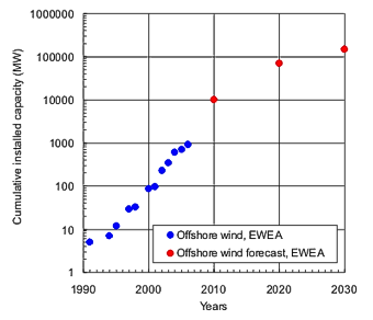
Fig. 1 – European offshore wind energy growth. (The offshore wind data comes from the European Wind Energy Association).
In order to perform an economic assessment and predict future costs of farms, an estimate of the growth rate is required. Figure 1 shows the current exponential growth in European offshore wind energy and the predicted growth over the coming decades. This leads to the following question.
Is this sort of growth possible for tidal or wave energy and if so how long will it last?
Only the future will tell, but in order to perform economic assessments it must be assumed that there is an analogy between the past growth of offshore wind technology and the future growth of the closely related marine renewable energy technologies.
In order to predict future costs of farms, it is common practice to assume a learning rate. A basic experience curve can be expressed as:
where CCum is the cost per unit; C0 the cost of the first unit produced; X is cumulative (unit) production; b is the experience index; PR the progress ratio and LR the learning rate. For example, a PR of 85% equates to a learning rate of 15% and therefore a 15% reduction in cost for each doubling of cumulative capacity. An assessment of the reduction of the intial farm start costs (turnkey costs) is made in Figure 2. This analysis suggests that a 60% reduction in initial farm costs may be possible over 20 years.
Fig. 2 – The possibilities for reduction in start costs based on different progress rates and exponential growth rates.
Further work within SERG includes the addition of more components to generate more complex economic models, including factors such as:
- effect of load factors
- capital discount rates
- O&M costs
- farm life
- decommissioning costs
Economic models are required for optimisation studies. Furthermore, their data can be used in other investigations such as assessments of socio-economic benefits.
Optimisation
Fig. 1 – Schematic sketch marine current energy converter.
Optimisation of marine current energy converters is a device- and location-specific problem and is constrained by large numbers of parameters. The initial studies within the research group have focused on small parts of a particular design such as the blade geometry or the effect of device orientation in the tidal flow.
However, more general global optimisation studies could require:
- forecasts of the available resource
- validated model of the device
- validated model of assessing wake interaction effects within a farm
- method of estimating costs
Optimisation is also dynamic problem and constantly varying as the markets change. A design produced one year may not represent the optimum design another year as prices may have changed, such as the cost of energy or materials.